Fitting Exercise

First to install packages

library(here)

here() starts at /Users/rebeccabasta/Desktop/EstherPalmer-portfolio

library(dplyr)

Attaching package: 'dplyr'

The following objects are masked from 'package:stats':

    filter, lag

The following objects are masked from 'package:base':

    intersect, setdiff, setequal, union

library(ggplot2)
library(tidymodels)

── Attaching packages ────────────────────────────────────── tidymodels 1.4.1 ──

✔ broom        1.0.12     ✔ rsample      1.3.2 
✔ dials        1.4.2      ✔ tailor       0.1.0 
✔ infer        1.1.0      ✔ tidyr        1.3.2 
✔ modeldata    1.5.1      ✔ tune         2.0.1 
✔ parsnip      1.4.1      ✔ workflows    1.3.0 
✔ purrr        1.2.1      ✔ workflowsets 1.1.1 
✔ recipes      1.3.1      ✔ yardstick    1.3.2 

── Conflicts ───────────────────────────────────────── tidymodels_conflicts() ──
✖ purrr::discard() masks scales::discard()
✖ dplyr::filter()  masks stats::filter()
✖ dplyr::lag()     masks stats::lag()
✖ recipes::step()  masks stats::step()

Then to load data

data_location <- here::here("fitting-exercise", "Mavoglurant_A2121_nmpk.csv")
df <- read.csv(data_location)

Plotting outcome (DV) as a function of time colored by dose and using ID as a grouping factor

p1 <- ggplot(df, aes(x=TIME, y=DV, group=ID, color=DOSE)) + geom_line()
plot(p1)

remove all OCC=2 entries, keep only OCC=1

df2 <- subset(df, (OCC == 1))

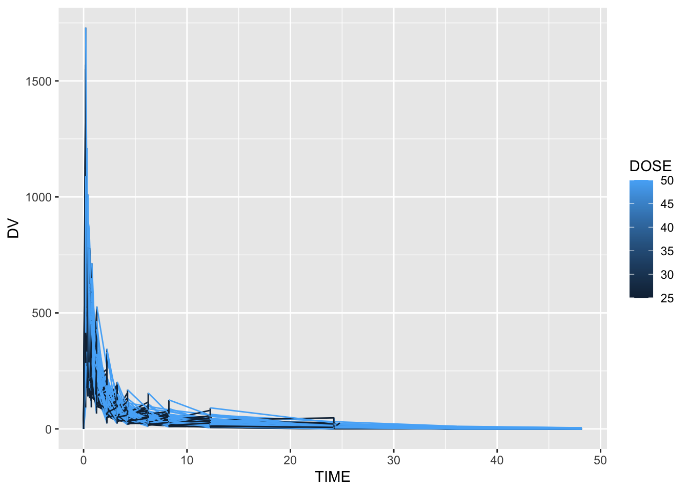
Exclude all Time=0, found sum of DV for each ID, create a new data frame with only time 0 and a new variable Y that contains amount of drug delivered over the whole experiment

df3 <- subset(df2, (TIME != 0))
df4 <- df3 %>% group_by(ID) %>% summarise(Y = sum(DV))
df5 <- subset(df2, (TIME == 0))
df6 <- left_join(x=df5, y=df4, by=c("ID"))

Keep only variables Y, Dose, Age, Sex, Race, WT, HT. Convert Race and Sex to factors

df7 <- select(df6,Y, DOSE, AGE, SEX, RACE, WT, HT)
df7$SEX <- as.factor(df7$SEX)
df7$RACE <- as.factor(df7$RACE)

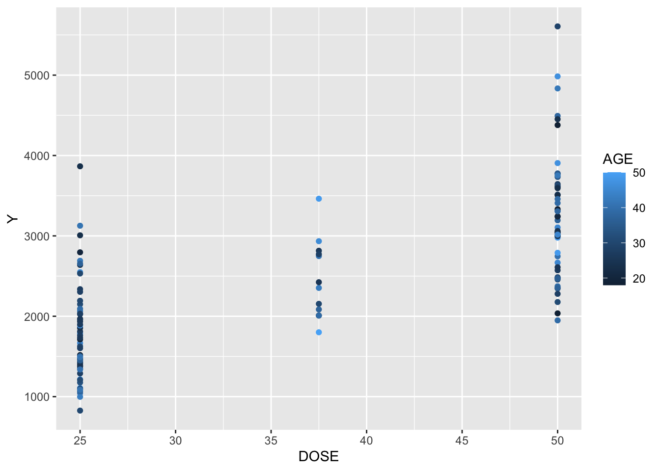
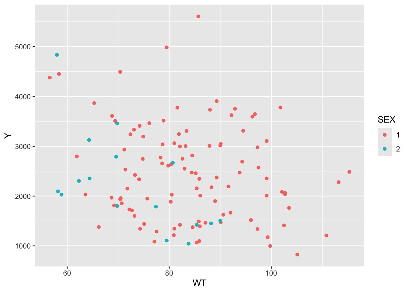
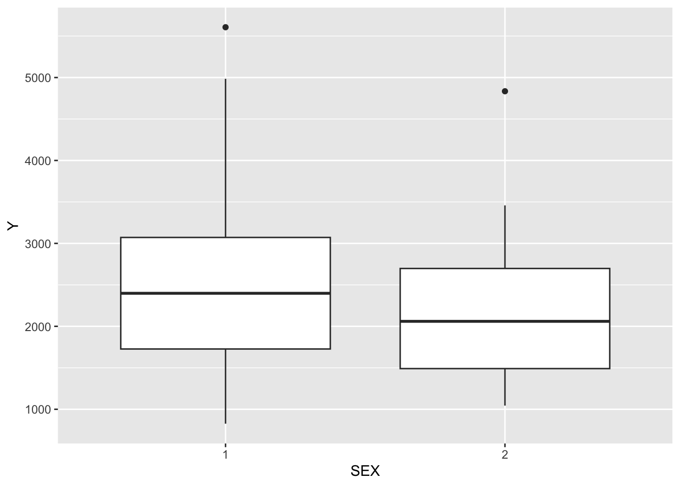
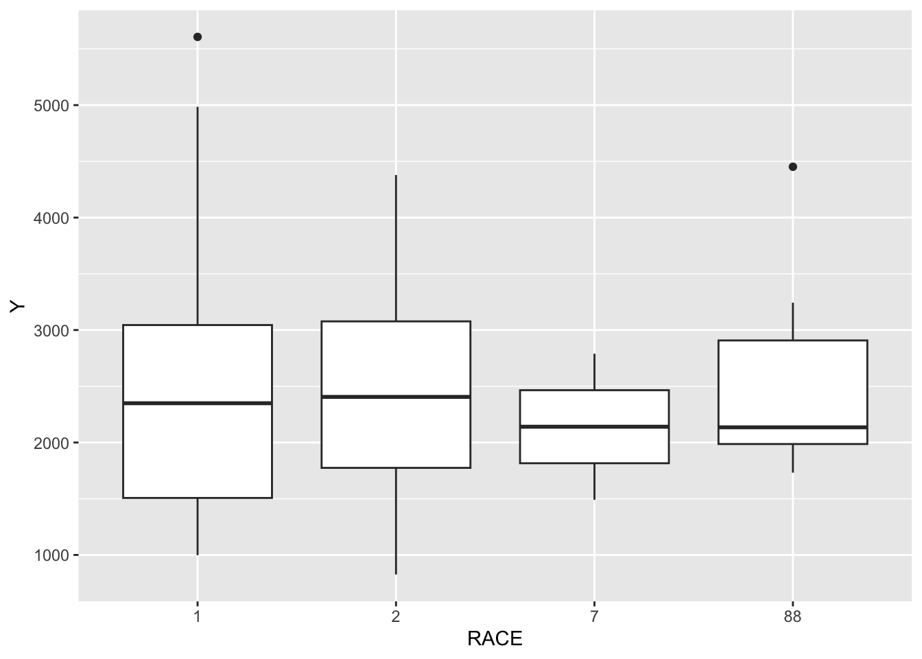
Plots depicting: dose and Y colored by Age Y and weight colored by Sex boxplot of Y by sex boxplot of Y by race

summary(df7)

       Y               DOSE            AGE        SEX     RACE   
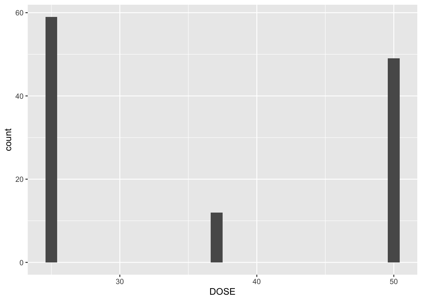
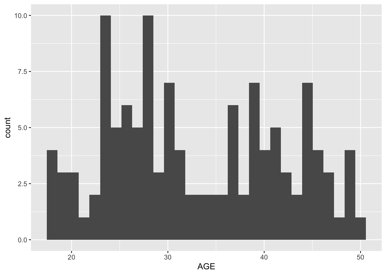
 Min.   : 826.4   Min.   :25.00   Min.   :18.00   1:104   1 :74  
 1st Qu.:1700.5   1st Qu.:25.00   1st Qu.:26.00   2: 16   2 :36  
 Median :2349.1   Median :37.50   Median :31.00           7 : 2  
 Mean   :2445.4   Mean   :36.46   Mean   :33.00           88: 8  
 3rd Qu.:3050.2   3rd Qu.:50.00   3rd Qu.:40.25                  
 Max.   :5606.6   Max.   :50.00   Max.   :50.00                  
       WT               HT       
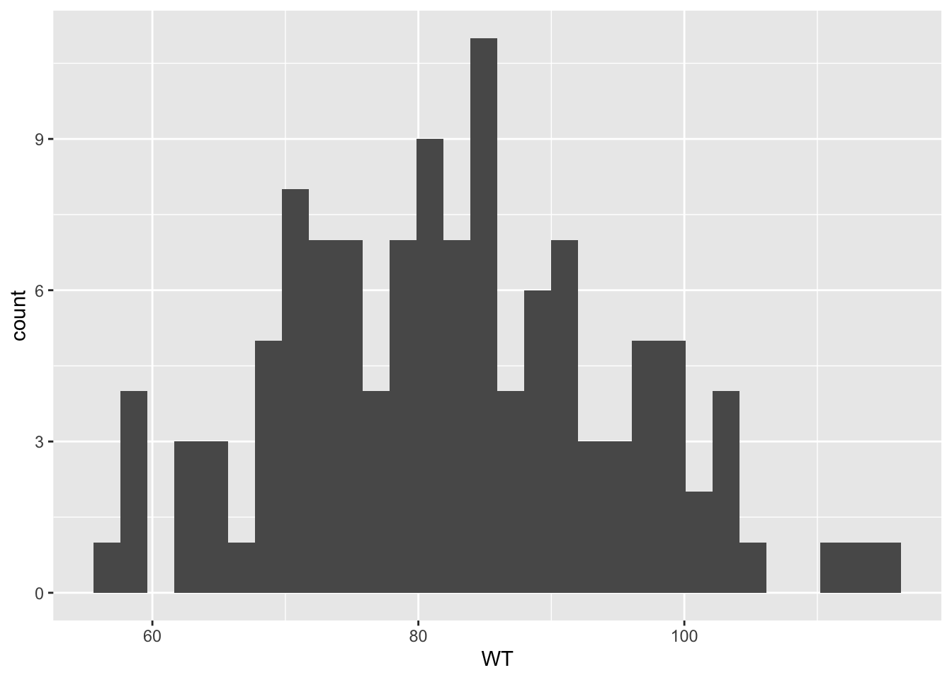
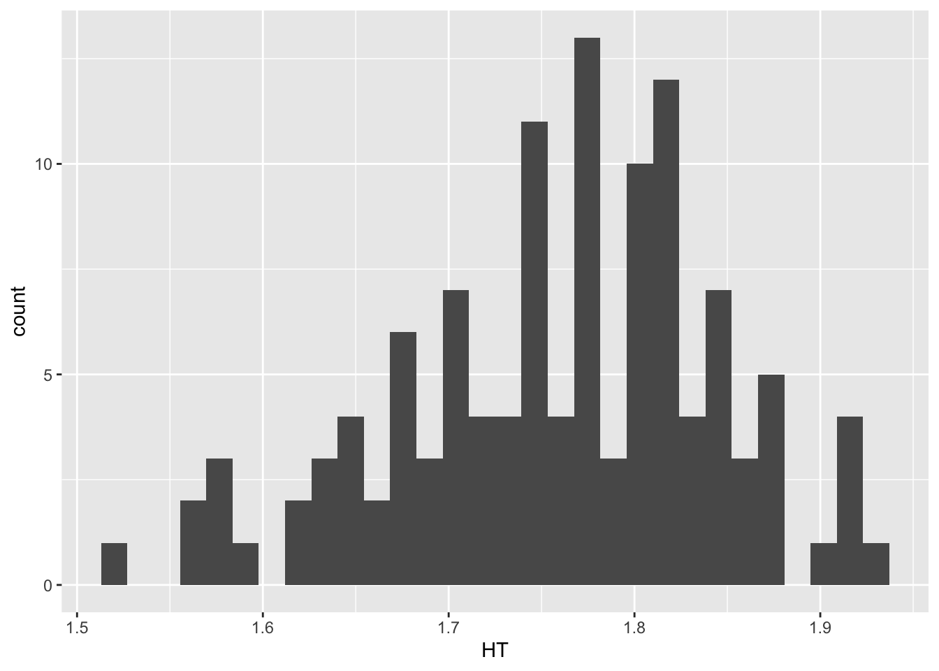
 Min.   : 56.60   Min.   :1.520  
 1st Qu.: 73.17   1st Qu.:1.700  
 Median : 82.10   Median :1.770  
 Mean   : 82.55   Mean   :1.759  
 3rd Qu.: 90.10   3rd Qu.:1.813  
 Max.   :115.30   Max.   :1.930  

p2 <- ggplot(df7, aes(x=DOSE, y=Y, color=AGE)) + geom_point()
plot(p2)

p3 <- ggplot(df7, aes(x=WT, y=Y, color=SEX)) + geom_point()
plot(p3)

p4 <- ggplot(df7, aes(x=SEX, y=Y)) + geom_boxplot()
plot(p4)

p5 <- ggplot(df7, aes(x=RACE, y=Y)) + geom_boxplot()
plot(p5)

hisDOSE <- ggplot(df7, aes(x=DOSE)) + geom_histogram()
plot(hisDOSE)

`stat_bin()` using `bins = 30`. Pick better value `binwidth`.

hisAGE <- ggplot(df7, aes(x=AGE)) + geom_histogram()
plot(hisAGE)

`stat_bin()` using `bins = 30`. Pick better value `binwidth`.

hisWT <- ggplot(df7, aes(x=WT)) + geom_histogram()
plot(hisWT)

`stat_bin()` using `bins = 30`. Pick better value `binwidth`.

hisHT <- ggplot(df7, aes(x=HT)) + geom_histogram()
plot(hisHT)

`stat_bin()` using `bins = 30`. Pick better value `binwidth`.

fit a linear model to Y using Dose and calculate RMSE/R2

lm_mod1 <- linear_reg()
lm_fit1 <- lm_mod1 %>% fit(Y ~ DOSE, data = df7)
lm_fit1

parsnip model object


Call:
stats::lm(formula = Y ~ DOSE, data = data)

Coefficients:
(Intercept)         DOSE  
     323.06        58.21  

pred1 <- predict(lm_fit1, df7) %>% bind_cols(df7)
met1 <- metrics(pred1, truth = Y, estimate = .pred)
met1

# A tibble: 3 × 3
  .metric .estimator .estimate
  <chr>   <chr>          <dbl>
1 rmse    standard     666.   
2 rsq     standard       0.516
3 mae     standard     517.   

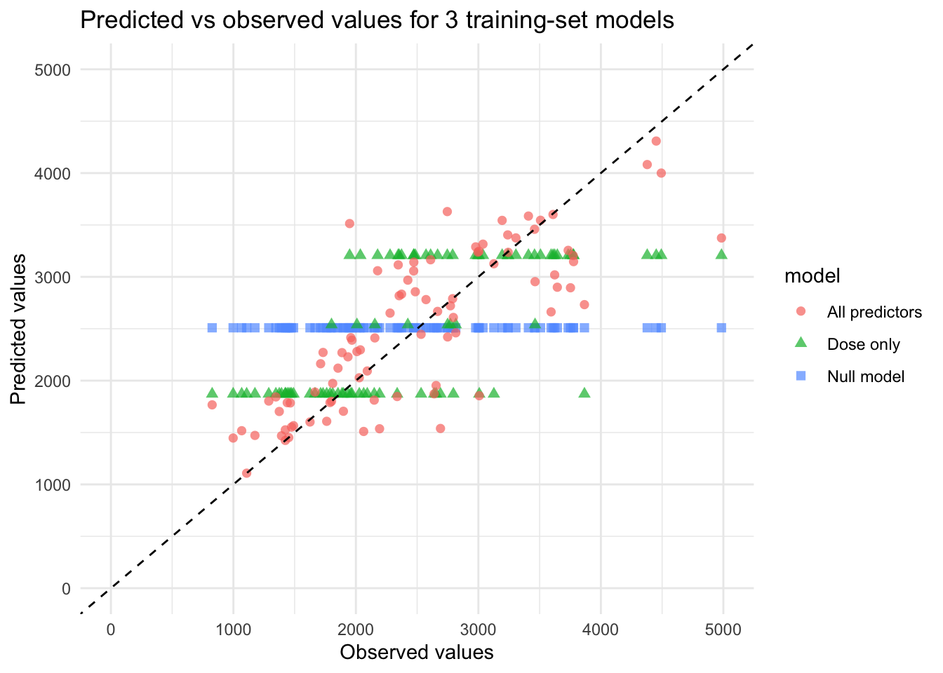
In this model dose has a coefficient of 58 which seems like a high number to me. (whenever my collaborators run models we get numbers like 1.2, although those are probably somewhat different models.) The R2 is .516 which is also decent in my opinion. I still have some issues figuring out how to interpret the RMSE and MAE though.

fit a linear model to Y using all predictors and calculate RMSE/R2

lm_mod2 <- linear_reg()
lm_fit2 <- lm_mod2 %>% fit(Y ~ DOSE * AGE * SEX * WT * HT * RACE, data = df7)
lm_fit2

parsnip model object


Call:
stats::lm(formula = Y ~ DOSE * AGE * SEX * WT * HT * RACE, data = data)

Coefficients:
               (Intercept)                        DOSE  
                 3.737e+05                  -1.280e+04  
                       AGE                        SEX2  
                -1.288e+04                  -3.292e+05  
                        WT                          HT  
                -4.527e+03                  -2.100e+05  
                     RACE2                       RACE7  
                -4.538e+05                  -1.828e+03  
                    RACE88                    DOSE:AGE  
                 5.751e+03                   4.358e+02  
                 DOSE:SEX2                    AGE:SEX2  
                -5.401e+02                   6.850e+03  
                   DOSE:WT                      AGE:WT  
                 1.561e+02                   1.545e+02  
                   SEX2:WT                     DOSE:HT  
                 1.827e+03                   7.201e+03  
                    AGE:HT                     SEX2:HT  
                 7.281e+03                   1.471e+05  
                     WT:HT                  DOSE:RACE2  
                 2.547e+03                   2.147e+04  
                DOSE:RACE7                 DOSE:RACE88  
                 6.996e+01                   1.436e+02  
                 AGE:RACE2                   AGE:RACE7  
                 1.602e+04                          NA  
                AGE:RACE88                  SEX2:RACE2  
                -1.934e+02                   2.501e+04  
                SEX2:RACE7                 SEX2:RACE88  
                        NA                   3.370e+03  
                  WT:RACE2                    WT:RACE7  
                 6.087e+03                          NA  
                 WT:RACE88                    HT:RACE2  
                 3.225e+01                   2.675e+05  
                  HT:RACE7                   HT:RACE88  
                        NA                  -2.314e+03  
             DOSE:AGE:SEX2                 DOSE:AGE:WT  
                -4.216e+01                  -5.229e+00  
              DOSE:SEX2:WT                 AGE:SEX2:WT  
                 2.333e+00                  -1.251e+01  
               DOSE:AGE:HT                DOSE:SEX2:HT  
                -2.446e+02                   1.332e+03  
               AGE:SEX2:HT                  DOSE:WT:HT  
                -2.849e+03                  -8.741e+01  
                 AGE:WT:HT                  SEX2:WT:HT  
                -8.735e+01                  -8.342e+02  
            DOSE:AGE:RACE2              DOSE:AGE:RACE7  
                -7.186e+02                          NA  
           DOSE:AGE:RACE88             DOSE:SEX2:RACE2  
                 2.775e+00                          NA  
           DOSE:SEX2:RACE7            DOSE:SEX2:RACE88  
                        NA                          NA  
            AGE:SEX2:RACE2              AGE:SEX2:RACE7  
                -1.493e+02                          NA  
           AGE:SEX2:RACE88               DOSE:WT:RACE2  
                        NA                  -2.718e+02  
             DOSE:WT:RACE7              DOSE:WT:RACE88  
                        NA                  -2.516e+00  
              AGE:WT:RACE2                AGE:WT:RACE7  
                -2.064e+02                          NA  
             AGE:WT:RACE88               SEX2:WT:RACE2  
                        NA                  -2.356e+02  
             SEX2:WT:RACE7              SEX2:WT:RACE88  
                        NA                          NA  
             DOSE:HT:RACE2               DOSE:HT:RACE7  
                -1.230e+04                          NA  
            DOSE:HT:RACE88                AGE:HT:RACE2  
                        NA                  -9.464e+03  
              AGE:HT:RACE7               AGE:HT:RACE88  
                        NA                          NA  
             SEX2:HT:RACE2               SEX2:HT:RACE7  
                        NA                          NA  
            SEX2:HT:RACE88                 WT:HT:RACE2  
                        NA                  -3.565e+03  
               WT:HT:RACE7                WT:HT:RACE88  
                        NA                          NA  
          DOSE:AGE:SEX2:WT            DOSE:AGE:SEX2:HT  
                        NA                          NA  
            DOSE:AGE:WT:HT             DOSE:SEX2:WT:HT  
                 2.937e+00                          NA  
            AGE:SEX2:WT:HT         DOSE:AGE:SEX2:RACE2  
                        NA                          NA  
       DOSE:AGE:SEX2:RACE7        DOSE:AGE:SEX2:RACE88  
                        NA                          NA  
         DOSE:AGE:WT:RACE2           DOSE:AGE:WT:RACE7  
                 8.881e+00                          NA  
        DOSE:AGE:WT:RACE88          DOSE:SEX2:WT:RACE2  
                        NA                          NA  
        DOSE:SEX2:WT:RACE7         DOSE:SEX2:WT:RACE88  
                        NA                          NA  
         AGE:SEX2:WT:RACE2           AGE:SEX2:WT:RACE7  
                        NA                          NA  
        AGE:SEX2:WT:RACE88           DOSE:AGE:HT:RACE2  
                        NA                   4.143e+02  
         DOSE:AGE:HT:RACE7          DOSE:AGE:HT:RACE88  
                        NA                          NA  
        DOSE:SEX2:HT:RACE2          DOSE:SEX2:HT:RACE7  
                        NA                          NA  
       DOSE:SEX2:HT:RACE88           AGE:SEX2:HT:RACE2  
                        NA                          NA  
         AGE:SEX2:HT:RACE7          AGE:SEX2:HT:RACE88  
                        NA                          NA  
          DOSE:WT:HT:RACE2            DOSE:WT:HT:RACE7  
                 1.552e+02                          NA  
         DOSE:WT:HT:RACE88             AGE:WT:HT:RACE2  
                        NA                   1.214e+02  
           AGE:WT:HT:RACE7            AGE:WT:HT:RACE88  
                        NA                          NA  
          SEX2:WT:HT:RACE2            SEX2:WT:HT:RACE7  
                        NA                          NA  
         SEX2:WT:HT:RACE88         DOSE:AGE:SEX2:WT:HT  
                        NA                          NA  
    DOSE:AGE:SEX2:WT:RACE2      DOSE:AGE:SEX2:WT:RACE7  
                        NA                          NA  
   DOSE:AGE:SEX2:WT:RACE88      DOSE:AGE:SEX2:HT:RACE2  
                        NA                          NA  
    DOSE:AGE:SEX2:HT:RACE7     DOSE:AGE:SEX2:HT:RACE88  
                        NA                          NA  
      DOSE:AGE:WT:HT:RACE2        DOSE:AGE:WT:HT:RACE7  
                -5.107e+00                          NA  
     DOSE:AGE:WT:HT:RACE88       DOSE:SEX2:WT:HT:RACE2  
                        NA                          NA  
     DOSE:SEX2:WT:HT:RACE7      DOSE:SEX2:WT:HT:RACE88  
                        NA                          NA  
      AGE:SEX2:WT:HT:RACE2        AGE:SEX2:WT:HT:RACE7  
                        NA                          NA  
     AGE:SEX2:WT:HT:RACE88   DOSE:AGE:SEX2:WT:HT:RACE2  
                        NA                          NA  
 DOSE:AGE:SEX2:WT:HT:RACE7  DOSE:AGE:SEX2:WT:HT:RACE88  
                        NA                          NA  

pred2 <- predict(lm_fit2, df7) %>% bind_cols(df7)

Warning in predict.lm(object = object$fit, newdata = new_data, type =
"response", : prediction from rank-deficient fit; consider predict(.,
rankdeficient="NA")

met2 <- metrics(pred2, truth = Y, estimate = .pred)
met2

# A tibble: 3 × 3
  .metric .estimator .estimate
  <chr>   <chr>          <dbl>
1 rmse    standard     475.   
2 rsq     standard       0.754
3 mae     standard     316.   

This one has a lower RMSE/MAE and a higher R2, so I can conclude that it is probably a better model than the first.

fit a linear model to SEX using Dose, and one using all predictors, and calculate ROC-AUC

lm_mod3 <- logistic_reg()
lm_fit3 <- lm_mod3 %>% fit(SEX ~ DOSE, data = df7)
lm_fit3

parsnip model object


Call:  stats::glm(formula = SEX ~ DOSE, family = stats::binomial, data = data)

Coefficients:
(Intercept)         DOSE  
   -0.76482     -0.03175  

Degrees of Freedom: 119 Total (i.e. Null);  118 Residual
Null Deviance:      94.24 
Residual Deviance: 92.43    AIC: 96.43

pred3 <- predict(lm_fit3, df7, type = "prob") %>% bind_cols(df7)
roc_auc(pred3, truth = SEX, .pred_1)

# A tibble: 1 × 3
  .metric .estimator .estimate
  <chr>   <chr>          <dbl>
1 roc_auc binary         0.592

lm_mod4 <- logistic_reg()
lm_fit4 <- lm_mod4 %>% fit(SEX ~ DOSE * Y * AGE * WT * HT * RACE, data = df7)

Warning: glm.fit: algorithm did not converge

Warning: glm.fit: fitted probabilities numerically 0 or 1 occurred

lm_fit4

parsnip model object


Call:  stats::glm(formula = SEX ~ DOSE * Y * AGE * WT * HT * RACE, family = stats::binomial, 
    data = data)

Coefficients:
            (Intercept)                     DOSE                        Y  
             -1.198e+05                1.894e+03                5.403e+01  
                    AGE                       WT                       HT  
              1.233e+03                1.353e+03                6.285e+04  
                  RACE2                    RACE7                   RACE88  
              1.321e+12                1.924e+02                2.296e+03  
                 DOSE:Y                 DOSE:AGE                    Y:AGE  
             -1.009e+00               -1.037e+01               -4.375e-01  
                DOSE:WT                     Y:WT                   AGE:WT  
             -2.176e+01               -6.039e-01               -1.290e+01  
                DOSE:HT                     Y:HT                   AGE:HT  
             -9.928e+02               -2.722e+01               -5.610e+02  
                  WT:HT               DOSE:RACE2               DOSE:RACE7  
             -7.069e+02               -5.282e+10               -6.955e+00  
            DOSE:RACE88                  Y:RACE2                  Y:RACE7  
             -1.732e+00               -2.175e+08                       NA  
               Y:RACE88                AGE:RACE2                AGE:RACE7  
             -1.002e+00                1.362e+10                       NA  
             AGE:RACE88                 WT:RACE2                 WT:RACE7  
              1.252e+01               -1.419e+10                       NA  
              WT:RACE88                 HT:RACE2                 HT:RACE7  
             -1.227e+01               -6.982e+11                       NA  
              HT:RACE88               DOSE:Y:AGE                DOSE:Y:WT  
             -1.498e+02                6.794e-03                1.131e-02  
            DOSE:AGE:WT                 Y:AGE:WT                DOSE:Y:HT  
              1.070e-01                4.634e-03                5.088e-01  
            DOSE:AGE:HT                 Y:AGE:HT               DOSE:WT:HT  
              3.645e+00                1.505e-01                1.135e+01  
                Y:WT:HT                AGE:WT:HT             DOSE:Y:RACE2  
              3.023e-01                5.704e+00                8.699e+06  
           DOSE:Y:RACE7            DOSE:Y:RACE88           DOSE:AGE:RACE2  
                     NA                1.623e-02               -5.449e+08  
         DOSE:AGE:RACE7          DOSE:AGE:RACE88              Y:AGE:RACE2  
                     NA               -5.302e-01               -6.826e+06  
            Y:AGE:RACE7             Y:AGE:RACE88            DOSE:WT:RACE2  
                     NA                       NA                5.678e+08  
          DOSE:WT:RACE7           DOSE:WT:RACE88               Y:WT:RACE2  
                     NA                       NA                2.536e+06  
             Y:WT:RACE7              Y:WT:RACE88             AGE:WT:RACE2  
                     NA                       NA               -2.310e+08  
           AGE:WT:RACE7            AGE:WT:RACE88            DOSE:HT:RACE2  
                     NA                       NA                2.793e+10  
          DOSE:HT:RACE7           DOSE:HT:RACE88               Y:HT:RACE2  
                     NA                       NA                1.127e+08  
             Y:HT:RACE7              Y:HT:RACE88             AGE:HT:RACE2  
                     NA                       NA               -8.945e+09  
           AGE:HT:RACE7            AGE:HT:RACE88              WT:HT:RACE2  
                     NA                       NA                7.528e+09  
            WT:HT:RACE7             WT:HT:RACE88            DOSE:Y:AGE:WT  
                     NA                       NA               -7.177e-05  
          DOSE:Y:AGE:HT             DOSE:Y:WT:HT           DOSE:AGE:WT:HT  
             -2.030e-03               -5.662e-03               -3.393e-02  
            Y:AGE:WT:HT         DOSE:Y:AGE:RACE2         DOSE:Y:AGE:RACE7  
             -1.506e-03                2.731e+05                       NA  
      DOSE:Y:AGE:RACE88          DOSE:Y:WT:RACE2          DOSE:Y:WT:RACE7  
                     NA               -1.014e+05                       NA  
       DOSE:Y:WT:RACE88        DOSE:AGE:WT:RACE2        DOSE:AGE:WT:RACE7  
                     NA                9.240e+06                       NA  
     DOSE:AGE:WT:RACE88           Y:AGE:WT:RACE2           Y:AGE:WT:RACE7  
                     NA                8.958e+04                       NA  
        Y:AGE:WT:RACE88          DOSE:Y:HT:RACE2          DOSE:Y:HT:RACE7  
                     NA               -4.507e+06                       NA  
       DOSE:Y:HT:RACE88        DOSE:AGE:HT:RACE2        DOSE:AGE:HT:RACE7  
                     NA                3.578e+08                       NA  
     DOSE:AGE:HT:RACE88           Y:AGE:HT:RACE2           Y:AGE:HT:RACE7  
                     NA                4.099e+06                       NA  
        Y:AGE:HT:RACE88         DOSE:WT:HT:RACE2         DOSE:WT:HT:RACE7  
                     NA               -3.011e+08                       NA  
      DOSE:WT:HT:RACE88            Y:WT:HT:RACE2            Y:WT:HT:RACE7  
                     NA               -1.335e+06                       NA  
         Y:WT:HT:RACE88          AGE:WT:HT:RACE2          AGE:WT:HT:RACE7  
                     NA                1.427e+08                       NA  
       AGE:WT:HT:RACE88         DOSE:Y:AGE:WT:HT      DOSE:Y:AGE:WT:RACE2  
                     NA                1.959e-05               -3.583e+03  
    DOSE:Y:AGE:WT:RACE7     DOSE:Y:AGE:WT:RACE88      DOSE:Y:AGE:HT:RACE2  
                     NA                       NA               -1.640e+05  
    DOSE:Y:AGE:HT:RACE7     DOSE:Y:AGE:HT:RACE88       DOSE:Y:WT:HT:RACE2  
                     NA                       NA                5.340e+04  
     DOSE:Y:WT:HT:RACE7      DOSE:Y:WT:HT:RACE88     DOSE:AGE:WT:HT:RACE2  
                     NA                       NA               -5.709e+06  
   DOSE:AGE:WT:HT:RACE7    DOSE:AGE:WT:HT:RACE88        Y:AGE:WT:HT:RACE2  
                     NA                       NA               -5.273e+04  
      Y:AGE:WT:HT:RACE7       Y:AGE:WT:HT:RACE88   DOSE:Y:AGE:WT:HT:RACE2  
                     NA                       NA                2.109e+03  
 DOSE:Y:AGE:WT:HT:RACE7  DOSE:Y:AGE:WT:HT:RACE88  
                     NA                       NA  

Degrees of Freedom: 119 Total (i.e. Null);  46 Residual
Null Deviance:      94.24 
Residual Deviance: 3.271e-09    AIC: 148

pred4 <- predict(lm_fit4, df7, type = "prob") %>% bind_cols(df7)
roc_auc(pred4, truth = SEX, .pred_1)

# A tibble: 1 × 3
  .metric .estimator .estimate
  <chr>   <chr>          <dbl>
1 roc_auc binary             1

The roc_auc is 1 for the last model which is super interesting. I guess that means that all the data put together are very good at predicting sex. This makes sense given that a lot of the things in the model are correlated with sex (height/weight, and doeses tend to be different for men/women). In model 3, dose alone had an ROC of .6, so it’s probably a decent predictor of sex.

random seed:

rngseed = 1234

remove race as a variable

df8 <- df7 %>% select(-RACE)

set seed and split data 75:25

set.seed(rngseed)

data_split  <- initial_split(df8, prop = 3/4)

train <- training(data_split)
test <- testing(data_split)

two linear models for Y (continuous outcome of interest) Model 1: dose as only pred Model 2: all predictors

set.seed(rngseed)
lm_mod5 <- linear_reg()
lm_fit5 <- lm_mod5 %>% fit(Y ~ DOSE, data = train)
lm_fit5

parsnip model object


Call:
stats::lm(formula = Y ~ DOSE, data = data)

Coefficients:
(Intercept)         DOSE  
     535.45        53.42  

pred5 <- predict(lm_fit5, train) %>% bind_cols(train)
met5 <- metrics(pred5, truth = Y, estimate = .pred)
met5

# A tibble: 3 × 3
  .metric .estimator .estimate
  <chr>   <chr>          <dbl>
1 rmse    standard     703.   
2 rsq     standard       0.451
3 mae     standard     546.   

lm_mod6 <- linear_reg()
lm_fit6 <- lm_mod6 %>% fit(Y ~ DOSE * AGE * SEX * WT * HT, data = train)
lm_fit6

parsnip model object


Call:
stats::lm(formula = Y ~ DOSE * AGE * SEX * WT * HT, data = data)

Coefficients:
        (Intercept)                 DOSE                  AGE  
          9.525e+04           -3.070e+03           -1.108e+03  
               SEX2                   WT                   HT  
          1.079e+05           -1.723e+03           -5.049e+04  
           DOSE:AGE            DOSE:SEX2             AGE:SEX2  
          8.184e+01            1.198e+03           -5.065e+03  
            DOSE:WT               AGE:WT              SEX2:WT  
          5.299e+01            3.454e+01            7.704e+02  
            DOSE:HT               AGE:HT              SEX2:HT  
          1.735e+03            5.416e+02           -5.277e+04  
              WT:HT        DOSE:AGE:SEX2          DOSE:AGE:WT  
          9.390e+02            2.381e+01           -1.531e+00  
       DOSE:SEX2:WT          AGE:SEX2:WT          DOSE:AGE:HT  
          2.727e+01           -1.869e+01           -4.453e+01  
       DOSE:SEX2:HT          AGE:SEX2:HT           DOSE:WT:HT  
         -2.680e+03            3.534e+03           -2.963e+01  
          AGE:WT:HT           SEX2:WT:HT     DOSE:AGE:SEX2:WT  
         -1.861e+01           -3.898e+02                   NA  
   DOSE:AGE:SEX2:HT       DOSE:AGE:WT:HT      DOSE:SEX2:WT:HT  
                 NA            8.471e-01                   NA  
     AGE:SEX2:WT:HT  DOSE:AGE:SEX2:WT:HT  
                 NA                   NA  

pred6 <- predict(lm_fit6, train) %>% bind_cols(train)

Warning in predict.lm(object = object$fit, newdata = new_data, type =
"response", : prediction from rank-deficient fit; consider predict(.,
rankdeficient="NA")

met6 <- metrics(pred6, truth = Y, estimate = .pred)
met6

# A tibble: 3 × 3
  .metric .estimator .estimate
  <chr>   <chr>          <dbl>
1 rmse    standard     578.   
2 rsq     standard       0.628
3 mae     standard     415.   

NM <- null_model(mode = "regression", engine = "parsnip")
NM_fit <- NM %>% fit(Y ~., data = train)
NM_fit

parsnip model object

Null Classification Model
Predicted Value: 2509.171 

pred7 <- predict(NM_fit, train) %>% bind_cols(train)
met7 <- rmse(pred7, truth = Y, estimate = .pred)
met7

# A tibble: 1 × 3
  .metric .estimator .estimate
  <chr>   <chr>          <dbl>
1 rmse    standard        948.

I set the random seed correctly, however my values are different from the ones we’re supposed to get. I got 948 for the null which is correct, 703 for model 1 (correct value 702), and 578 for model 2 (correct value 627). This does mean that model 2 is currently performing best as it has the lowest rmse

Now I need to do a 10-fold CV

folds <- vfold_cv(train, v = 10)
folds

#  10-fold cross-validation 
# A tibble: 10 × 2
   splits         id    
   <list>         <chr> 
 1 <split [81/9]> Fold01
 2 <split [81/9]> Fold02
 3 <split [81/9]> Fold03
 4 <split [81/9]> Fold04
 5 <split [81/9]> Fold05
 6 <split [81/9]> Fold06
 7 <split [81/9]> Fold07
 8 <split [81/9]> Fold08
 9 <split [81/9]> Fold09
10 <split [81/9]> Fold10

lm_wf1 <- workflow() %>% add_model(lm_mod5) %>% add_formula(Y ~ DOSE)
lm_fit_cv1 <- lm_wf1 %>% fit_resamples(folds)
lm_fit_cv1

# Resampling results
# 10-fold cross-validation 
# A tibble: 10 × 4
   splits         id     .metrics         .notes          
   <list>         <chr>  <list>           <list>          
 1 <split [81/9]> Fold01 <tibble [2 × 4]> <tibble [0 × 4]>
 2 <split [81/9]> Fold02 <tibble [2 × 4]> <tibble [0 × 4]>
 3 <split [81/9]> Fold03 <tibble [2 × 4]> <tibble [0 × 4]>
 4 <split [81/9]> Fold04 <tibble [2 × 4]> <tibble [0 × 4]>
 5 <split [81/9]> Fold05 <tibble [2 × 4]> <tibble [0 × 4]>
 6 <split [81/9]> Fold06 <tibble [2 × 4]> <tibble [0 × 4]>
 7 <split [81/9]> Fold07 <tibble [2 × 4]> <tibble [0 × 4]>
 8 <split [81/9]> Fold08 <tibble [2 × 4]> <tibble [0 × 4]>
 9 <split [81/9]> Fold09 <tibble [2 × 4]> <tibble [0 × 4]>
10 <split [81/9]> Fold10 <tibble [2 × 4]> <tibble [0 × 4]>

collect_metrics(lm_fit_cv1)

# A tibble: 2 × 6
  .metric .estimator    mean     n std_err .config        
  <chr>   <chr>        <dbl> <int>   <dbl> <chr>          
1 rmse    standard   691.       10 67.5    pre0_mod0_post0
2 rsq     standard     0.512    10  0.0592 pre0_mod0_post0

lm_wf2 <- workflow() %>% add_model(lm_mod5) %>% add_formula(Y ~ DOSE * AGE * SEX * WT * HT)
lm_fit_cv2 <- lm_wf2 %>% fit_resamples(folds)

→ A | warning: prediction from rank-deficient fit; consider predict(., rankdeficient="NA")

There were issues with some computations   A: x1

There were issues with some computations   A: x10

lm_fit_cv2

# Resampling results
# 10-fold cross-validation 
# A tibble: 10 × 4
   splits         id     .metrics         .notes          
   <list>         <chr>  <list>           <list>          
 1 <split [81/9]> Fold01 <tibble [2 × 4]> <tibble [1 × 4]>
 2 <split [81/9]> Fold02 <tibble [2 × 4]> <tibble [1 × 4]>
 3 <split [81/9]> Fold03 <tibble [2 × 4]> <tibble [1 × 4]>
 4 <split [81/9]> Fold04 <tibble [2 × 4]> <tibble [1 × 4]>
 5 <split [81/9]> Fold05 <tibble [2 × 4]> <tibble [1 × 4]>
 6 <split [81/9]> Fold06 <tibble [2 × 4]> <tibble [1 × 4]>
 7 <split [81/9]> Fold07 <tibble [2 × 4]> <tibble [1 × 4]>
 8 <split [81/9]> Fold08 <tibble [2 × 4]> <tibble [1 × 4]>
 9 <split [81/9]> Fold09 <tibble [2 × 4]> <tibble [1 × 4]>
10 <split [81/9]> Fold10 <tibble [2 × 4]> <tibble [1 × 4]>

There were issues with some computations:

  - Warning(s) x10: prediction from rank-deficient fit; consider predict(., rankdefic...

Run `show_notes(.Last.tune.result)` for more information.

collect_metrics(lm_fit_cv2)

# A tibble: 2 × 6
  .metric .estimator     mean     n   std_err .config        
  <chr>   <chr>         <dbl> <int>     <dbl> <chr>          
1 rmse    standard   7599.       10 5695.     pre0_mod0_post0
2 rsq     standard      0.347    10    0.0807 pre0_mod0_post0

NM_wf <- workflow() %>% add_model(NM) %>% add_formula(Y ~ .)
NM_fit_cv <- NM_wf %>% fit_resamples(folds)

→ A | warning: A correlation computation is required, but `estimate` is constant and has 0
               standard deviation, resulting in a divide by 0 error. `NA` will be returned.

NM_fit_cv

# Resampling results
# 10-fold cross-validation 
# A tibble: 10 × 4
   splits         id     .metrics         .notes          
   <list>         <chr>  <list>           <list>          
 1 <split [81/9]> Fold01 <tibble [2 × 4]> <tibble [1 × 4]>
 2 <split [81/9]> Fold02 <tibble [2 × 4]> <tibble [1 × 4]>
 3 <split [81/9]> Fold03 <tibble [2 × 4]> <tibble [1 × 4]>
 4 <split [81/9]> Fold04 <tibble [2 × 4]> <tibble [1 × 4]>
 5 <split [81/9]> Fold05 <tibble [2 × 4]> <tibble [1 × 4]>
 6 <split [81/9]> Fold06 <tibble [2 × 4]> <tibble [1 × 4]>
 7 <split [81/9]> Fold07 <tibble [2 × 4]> <tibble [1 × 4]>
 8 <split [81/9]> Fold08 <tibble [2 × 4]> <tibble [1 × 4]>
 9 <split [81/9]> Fold09 <tibble [2 × 4]> <tibble [1 × 4]>
10 <split [81/9]> Fold10 <tibble [2 × 4]> <tibble [1 × 4]>

There were issues with some computations:

  - Warning(s) x10: A correlation computation is required, but `estimate` is constant...

Run `show_notes(.Last.tune.result)` for more information.

collect_metrics(NM_fit_cv)

# A tibble: 2 × 6
  .metric .estimator  mean     n std_err .config        
  <chr>   <chr>      <dbl> <int>   <dbl> <chr>          
1 rmse    standard    933.    10    76.7 pre0_mod0_post0
2 rsq     standard    NaN      0    NA   pre0_mod0_post0

Well the rmse for the null model was similar but different at 943, SE at 66.2. RMSE for the second model with the full formula was much worse at 2003, while rmse for the Y~DOSE model was 687.

Now I need a different random seed

set.seed(347)
folds2 <- vfold_cv(train, v = 10)
folds2

#  10-fold cross-validation 
# A tibble: 10 × 2
   splits         id    
   <list>         <chr> 
 1 <split [81/9]> Fold01
 2 <split [81/9]> Fold02
 3 <split [81/9]> Fold03
 4 <split [81/9]> Fold04
 5 <split [81/9]> Fold05
 6 <split [81/9]> Fold06
 7 <split [81/9]> Fold07
 8 <split [81/9]> Fold08
 9 <split [81/9]> Fold09
10 <split [81/9]> Fold10

lm_wf3 <- workflow() %>% add_model(lm_mod5) %>% add_formula(Y ~ DOSE)
lm_fit_cv3 <- lm_wf3 %>% fit_resamples(folds2)
lm_fit_cv3

# Resampling results
# 10-fold cross-validation 
# A tibble: 10 × 4
   splits         id     .metrics         .notes          
   <list>         <chr>  <list>           <list>          
 1 <split [81/9]> Fold01 <tibble [2 × 4]> <tibble [0 × 4]>
 2 <split [81/9]> Fold02 <tibble [2 × 4]> <tibble [0 × 4]>
 3 <split [81/9]> Fold03 <tibble [2 × 4]> <tibble [0 × 4]>
 4 <split [81/9]> Fold04 <tibble [2 × 4]> <tibble [0 × 4]>
 5 <split [81/9]> Fold05 <tibble [2 × 4]> <tibble [0 × 4]>
 6 <split [81/9]> Fold06 <tibble [2 × 4]> <tibble [0 × 4]>
 7 <split [81/9]> Fold07 <tibble [2 × 4]> <tibble [0 × 4]>
 8 <split [81/9]> Fold08 <tibble [2 × 4]> <tibble [0 × 4]>
 9 <split [81/9]> Fold09 <tibble [2 × 4]> <tibble [0 × 4]>
10 <split [81/9]> Fold10 <tibble [2 × 4]> <tibble [0 × 4]>

collect_metrics(lm_fit_cv3)

# A tibble: 2 × 6
  .metric .estimator    mean     n std_err .config        
  <chr>   <chr>        <dbl> <int>   <dbl> <chr>          
1 rmse    standard   684.       10 67.4    pre0_mod0_post0
2 rsq     standard     0.504    10  0.0722 pre0_mod0_post0

lm_wf4 <- workflow() %>% add_model(lm_mod5) %>% add_formula(Y ~ DOSE * AGE * SEX * WT * HT)
lm_fit_cv4 <- lm_wf4 %>% fit_resamples(folds2)

→ A | warning: prediction from rank-deficient fit; consider predict(., rankdeficient="NA")

lm_fit_cv4

# Resampling results
# 10-fold cross-validation 
# A tibble: 10 × 4
   splits         id     .metrics         .notes          
   <list>         <chr>  <list>           <list>          
 1 <split [81/9]> Fold01 <tibble [2 × 4]> <tibble [1 × 4]>
 2 <split [81/9]> Fold02 <tibble [2 × 4]> <tibble [1 × 4]>
 3 <split [81/9]> Fold03 <tibble [2 × 4]> <tibble [1 × 4]>
 4 <split [81/9]> Fold04 <tibble [2 × 4]> <tibble [1 × 4]>
 5 <split [81/9]> Fold05 <tibble [2 × 4]> <tibble [1 × 4]>
 6 <split [81/9]> Fold06 <tibble [2 × 4]> <tibble [1 × 4]>
 7 <split [81/9]> Fold07 <tibble [2 × 4]> <tibble [1 × 4]>
 8 <split [81/9]> Fold08 <tibble [2 × 4]> <tibble [1 × 4]>
 9 <split [81/9]> Fold09 <tibble [2 × 4]> <tibble [1 × 4]>
10 <split [81/9]> Fold10 <tibble [2 × 4]> <tibble [1 × 4]>

There were issues with some computations:

  - Warning(s) x10: prediction from rank-deficient fit; consider predict(., rankdefic...

Run `show_notes(.Last.tune.result)` for more information.

collect_metrics(lm_fit_cv2)

# A tibble: 2 × 6
  .metric .estimator     mean     n   std_err .config        
  <chr>   <chr>         <dbl> <int>     <dbl> <chr>          
1 rmse    standard   7599.       10 5695.     pre0_mod0_post0
2 rsq     standard      0.347    10    0.0807 pre0_mod0_post0

NM_wf2 <- workflow() %>% add_model(NM) %>% add_formula(Y ~ .)
NM_fit_cv2 <- NM_wf2 %>% fit_resamples(folds2)

→ A | warning: A correlation computation is required, but `estimate` is constant and has 0
               standard deviation, resulting in a divide by 0 error. `NA` will be returned.

There were issues with some computations   A: x1

There were issues with some computations   A: x10

NM_fit_cv2

# Resampling results
# 10-fold cross-validation 
# A tibble: 10 × 4
   splits         id     .metrics         .notes          
   <list>         <chr>  <list>           <list>          
 1 <split [81/9]> Fold01 <tibble [2 × 4]> <tibble [1 × 4]>
 2 <split [81/9]> Fold02 <tibble [2 × 4]> <tibble [1 × 4]>
 3 <split [81/9]> Fold03 <tibble [2 × 4]> <tibble [1 × 4]>
 4 <split [81/9]> Fold04 <tibble [2 × 4]> <tibble [1 × 4]>
 5 <split [81/9]> Fold05 <tibble [2 × 4]> <tibble [1 × 4]>
 6 <split [81/9]> Fold06 <tibble [2 × 4]> <tibble [1 × 4]>
 7 <split [81/9]> Fold07 <tibble [2 × 4]> <tibble [1 × 4]>
 8 <split [81/9]> Fold08 <tibble [2 × 4]> <tibble [1 × 4]>
 9 <split [81/9]> Fold09 <tibble [2 × 4]> <tibble [1 × 4]>
10 <split [81/9]> Fold10 <tibble [2 × 4]> <tibble [1 × 4]>

There were issues with some computations:

  - Warning(s) x10: A correlation computation is required, but `estimate` is constant...

Run `show_notes(.Last.tune.result)` for more information.

collect_metrics(NM_fit_cv2)

# A tibble: 2 × 6
  .metric .estimator  mean     n std_err .config        
  <chr>   <chr>      <dbl> <int>   <dbl> <chr>          
1 rmse    standard    938.    10    56.2 pre0_mod0_post0
2 rsq     standard    NaN      0    NA   pre0_mod0_post0

Null model is now at 938, similar but slightly different second model is still at 2003 First model is now at 684. Similar, but slightly different to the other random seed.

This section added by Rebecca Basta

Null Model Predictions

plot_null <- predict(NM_fit, train) %>%
  bind_cols(train %>% select(Y)) %>%
  mutate(model = "Null model")

Dose Model Predictions

plot_mod1 <- predict(lm_fit5, train) %>%
  bind_cols(train %>% select(Y)) %>%
  mutate(model = "Dose only")

All Predictor Model Predictions

plot_mod2 <- predict(lm_fit6, train) %>%
  bind_cols(train %>% select(Y)) %>%
  mutate(model = "All predictors")

Warning in predict.lm(object = object$fit, newdata = new_data, type =
"response", : prediction from rank-deficient fit; consider predict(.,
rankdeficient="NA")

Combine into One Dataframe

plot_df <- bind_rows(plot_null, plot_mod1, plot_mod2)

Predicted vs Observed Plot

p_pred_obs <- ggplot(plot_df, aes(x = Y, y = .pred, color = model, shape = model)) +
  geom_point(alpha = 0.7, size = 2) +
  geom_abline(slope = 1, intercept = 0, linetype = "dashed") +
  coord_cartesian(xlim = c(0, 5000), ylim = c(0, 5000)) +
  labs(
    x = "Observed values",
    y = "Predicted values",
    title = "Predicted vs observed values for 3 training-set models"
  ) +
  theme_minimal()

plot(p_pred_obs)