Future Exercise

library("dslabs")
str(gapminder)

'data.frame':   10545 obs. of  9 variables:
 $ country         : Factor w/ 185 levels "Albania","Algeria",..: 1 2 3 4 5 6 7 8 9 10 ...
 $ year            : int  1960 1960 1960 1960 1960 1960 1960 1960 1960 1960 ...
 $ infant_mortality: num  115.4 148.2 208 NA 59.9 ...
 $ life_expectancy : num  62.9 47.5 36 63 65.4 ...
 $ fertility       : num  6.19 7.65 7.32 4.43 3.11 4.55 4.82 3.45 2.7 5.57 ...
 $ population      : num  1636054 11124892 5270844 54681 20619075 ...
 $ gdp             : num  NA 1.38e+10 NA NA 1.08e+11 ...
 $ continent       : Factor w/ 5 levels "Africa","Americas",..: 4 1 1 2 2 3 2 5 4 3 ...
 $ region          : Factor w/ 22 levels "Australia and New Zealand",..: 19 11 10 2 15 21 2 1 22 21 ...

summary(gapminder)

                country           year      infant_mortality life_expectancy
 Albania            :   57   Min.   :1960   Min.   :  1.50   Min.   :13.20  
 Algeria            :   57   1st Qu.:1974   1st Qu.: 16.00   1st Qu.:57.50  
 Angola             :   57   Median :1988   Median : 41.50   Median :67.54  
 Antigua and Barbuda:   57   Mean   :1988   Mean   : 55.31   Mean   :64.81  
 Argentina          :   57   3rd Qu.:2002   3rd Qu.: 85.10   3rd Qu.:73.00  
 Armenia            :   57   Max.   :2016   Max.   :276.90   Max.   :83.90  
 (Other)            :10203                  NA's   :1453                    
   fertility       population             gdp               continent   
 Min.   :0.840   Min.   :3.124e+04   Min.   :4.040e+07   Africa  :2907  
 1st Qu.:2.200   1st Qu.:1.333e+06   1st Qu.:1.846e+09   Americas:2052  
 Median :3.750   Median :5.009e+06   Median :7.794e+09   Asia    :2679  
 Mean   :4.084   Mean   :2.701e+07   Mean   :1.480e+11   Europe  :2223  
 3rd Qu.:6.000   3rd Qu.:1.523e+07   3rd Qu.:5.540e+10   Oceania : 684  
 Max.   :9.220   Max.   :1.376e+09   Max.   :1.174e+13                  
 NA's   :187     NA's   :185         NA's   :2972                       
             region    
 Western Asia   :1026  
 Eastern Africa : 912  
 Western Africa : 912  
 Caribbean      : 741  
 South America  : 684  
 Southern Europe: 684  
 (Other)        :5586  

data(gapminder)

africadata <- subset(gapminder, (continent == "Africa"))
#creates a new dataframe from a subset of the old one where the continent is Africa
str(africadata)

'data.frame':   2907 obs. of  9 variables:
 $ country         : Factor w/ 185 levels "Albania","Algeria",..: 2 3 18 22 26 27 29 31 32 33 ...
 $ year            : int  1960 1960 1960 1960 1960 1960 1960 1960 1960 1960 ...
 $ infant_mortality: num  148 208 187 116 161 ...
 $ life_expectancy : num  47.5 36 38.3 50.3 35.2 ...
 $ fertility       : num  7.65 7.32 6.28 6.62 6.29 6.95 5.65 6.89 5.84 6.25 ...
 $ population      : num  11124892 5270844 2431620 524029 4829291 ...
 $ gdp             : num  1.38e+10 NA 6.22e+08 1.24e+08 5.97e+08 ...
 $ continent       : Factor w/ 5 levels "Africa","Americas",..: 1 1 1 1 1 1 1 1 1 1 ...
 $ region          : Factor w/ 22 levels "Australia and New Zealand",..: 11 10 20 17 20 5 10 20 10 10 ...

#Checks to make sure I have the correct number of observations

inf_LE <- data.frame(africadata$infant_mortality, africadata$life_expectancy)
#creates a new dataframe from these two columns of the africadata dataframe
#this one is for infant mortality and Life expectancy
str(inf_LE)

'data.frame':   2907 obs. of  2 variables:
 $ africadata.infant_mortality: num  148 208 187 116 161 ...
 $ africadata.life_expectancy : num  47.5 36 38.3 50.3 35.2 ...

#This checks to make sure I got it right

pop_LE <- data.frame(africadata$population, africadata$life_expectancy)
#This creates a new dataframe for population and life expectancy data
str(pop_LE)

'data.frame':   2907 obs. of  2 variables:
 $ africadata.population     : num  11124892 5270844 2431620 524029 4829291 ...
 $ africadata.life_expectancy: num  47.5 36 38.3 50.3 35.2 ...

#This checks that I have everything right

plot(inf_LE)

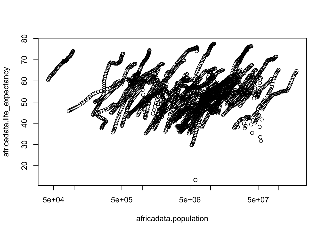
#plots this dataframe on a scatter plot
#plot(pop_LE$africadata.population, pop_LE$africadata.life_expectancy, log = "x")
#above is one option for generating the other scatter plot
plot(pop_LE, log = "x")

#here is a neater version
#the log function is where you can specify which axis should be in log, in this case population

My hypothesis for the streaks of data we see is that they are individual countries over time

year_inf <- data.frame(africadata$year, africadata$infant_mortality)
#this creates a matrix with year and infant mortality
year_inf[is.na(year_inf)] <- "A"
#this line rewrites the dataset, changing all NA's to A
missing <- subset(year_inf, (africadata.infant_mortality == "A"))
#this makes a new dataset with the subset function that pulls out all the years with A as a value
#This didn't work with NA which is why I changed it to A. Not the most elegant solution but it works
str(missing)

'data.frame':   226 obs. of  2 variables:
 $ africadata.year            : int  1960 1960 1960 1960 1960 1960 1960 1960 1960 1960 ...
 $ africadata.infant_mortality: chr  "A" "A" "A" "A" ...

#this line is for checking

year2000 <- subset(africadata, (year == "2000"))
#this creates a new data.frame with all the data from the year 2000 from africadata
str(year2000)

'data.frame':   51 obs. of  9 variables:
 $ country         : Factor w/ 185 levels "Albania","Algeria",..: 2 3 18 22 26 27 29 31 32 33 ...
 $ year            : int  2000 2000 2000 2000 2000 2000 2000 2000 2000 2000 ...
 $ infant_mortality: num  33.9 128.3 89.3 52.4 96.2 ...
 $ life_expectancy : num  73.3 52.3 57.2 47.6 52.6 46.7 54.3 68.4 45.3 51.5 ...
 $ fertility       : num  2.51 6.84 5.98 3.41 6.59 7.06 5.62 3.7 5.45 7.35 ...
 $ population      : num  31183658 15058638 6949366 1736579 11607944 ...
 $ gdp             : num  5.48e+10 9.13e+09 2.25e+09 5.63e+09 2.61e+09 ...
 $ continent       : Factor w/ 5 levels "Africa","Americas",..: 1 1 1 1 1 1 1 1 1 1 ...
 $ region          : Factor w/ 22 levels "Australia and New Zealand",..: 11 10 20 17 20 5 10 20 10 10 ...

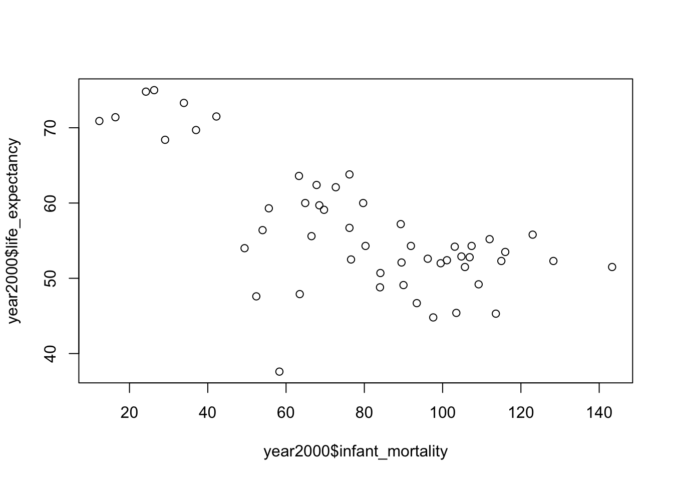
#this is for checking

plot(year2000$infant_mortality, year2000$life_expectancy)

plot(year2000$population, year2000$life_expectancy, log = "x")

These are the updated plots for the year 2000!

fit1 <- lm(year2000$life_expectancy ~ year2000$infant_mortality)
summary(fit1)

Call:
lm(formula = year2000$life_expectancy ~ year2000$infant_mortality)

Residuals:
     Min       1Q   Median       3Q      Max 
-22.6651  -3.7087   0.9914   4.0408   8.6817 

Coefficients:
                          Estimate Std. Error t value Pr(>|t|)    
(Intercept)               71.29331    2.42611  29.386  < 2e-16 ***
year2000$infant_mortality -0.18916    0.02869  -6.594 2.83e-08 ***
---
Signif. codes:  0 '***' 0.001 '**' 0.01 '*' 0.05 '.' 0.1 ' ' 1

Residual standard error: 6.221 on 49 degrees of freedom
Multiple R-squared:  0.4701,    Adjusted R-squared:  0.4593 
F-statistic: 43.48 on 1 and 49 DF,  p-value: 2.826e-08

fit2 <- lm(year2000$life_expectancy ~ year2000$population)
summary(fit2)

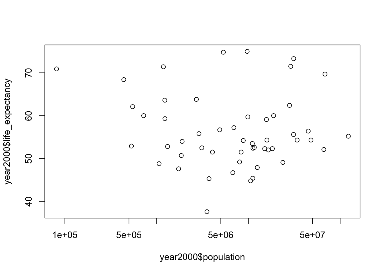
Call:
lm(formula = year2000$life_expectancy ~ year2000$population)

Residuals:
    Min      1Q  Median      3Q     Max 
-18.429  -4.602  -2.568   3.800  18.802 

Coefficients:
                     Estimate Std. Error t value Pr(>|t|)    
(Intercept)         5.593e+01  1.468e+00  38.097   <2e-16 ***
year2000$population 2.756e-08  5.459e-08   0.505    0.616    
---
Signif. codes:  0 '***' 0.001 '**' 0.01 '*' 0.05 '.' 0.1 ' ' 1

Residual standard error: 8.524 on 49 degrees of freedom
Multiple R-squared:  0.005176,  Adjusted R-squared:  -0.01513 
F-statistic: 0.2549 on 1 and 49 DF,  p-value: 0.6159

I used the help command to figure out what I needed to input into the lm command. It said the format was response ~ predictor. It also looked like I could set several responses and predictors.

This section is contributed by KATHERINELORUSSO

library(dplyr)

Attaching package: 'dplyr'

The following objects are masked from 'package:stats':

    filter, lag

The following objects are masked from 'package:base':

    intersect, setdiff, setequal, union

library(ggplot2)
str(us_contagious_diseases)

'data.frame':   16065 obs. of  6 variables:
 $ disease        : Factor w/ 7 levels "Hepatitis A",..: 1 1 1 1 1 1 1 1 1 1 ...
 $ state          : Factor w/ 51 levels "Alabama","Alaska",..: 1 1 1 1 1 1 1 1 1 1 ...
 $ year           : num  1966 1967 1968 1969 1970 ...
 $ weeks_reporting: num  50 49 52 49 51 51 45 45 45 46 ...
 $ count          : num  321 291 314 380 413 378 342 467 244 286 ...
 $ population     : num  3345787 3364130 3386068 3412450 3444165 ...

#str function was used to see how many observations and variables (16065 observations & 6 variables)
summary(us_contagious_diseases)

        disease            state            year      weeks_reporting
 Hepatitis A:2346   Alabama   :  315   Min.   :1928   Min.   : 0.00  
 Measles    :3825   Alaska    :  315   1st Qu.:1950   1st Qu.:31.00  
 Mumps      :1785   Arizona   :  315   Median :1975   Median :46.00  
 Pertussis  :2856   Arkansas  :  315   Mean   :1971   Mean   :37.38  
 Polio      :2091   California:  315   3rd Qu.:1990   3rd Qu.:50.00  
 Rubella    :1887   Colorado  :  315   Max.   :2011   Max.   :52.00  
 Smallpox   :1275   (Other)   :14175                                 
     count          population      
 Min.   :     0   Min.   :   86853  
 1st Qu.:     7   1st Qu.: 1018755  
 Median :    69   Median : 2749249  
 Mean   :  1493   Mean   : 4107584  
 3rd Qu.:   525   3rd Qu.: 4996229  
 Max.   :132342   Max.   :37607525  
                  NA's   :214       

#summary was used to view the variables and statistical values of the variables. 

GAmumps <- subset(us_contagious_diseases,state == "Georgia" & disease == "Mumps")
#I wanted to only look at Georgia & Mumps data, so I used the filter function and named it GAdmumps.
GAmumps2 <- data.frame(GAmumps$year, GAmumps$count)
#I then created a dataset of year and count for mumps. 
summary(GAmumps2)

  GAmumps.year  GAmumps.count  
 Min.   :1968   Min.   :  1.0  
 1st Qu.:1976   1st Qu.:  6.0  
 Median :1985   Median : 18.0  
 Mean   :1985   Mean   : 29.2  
 3rd Qu.:1994   3rd Qu.: 38.5  
 Max.   :2002   Max.   :103.0  

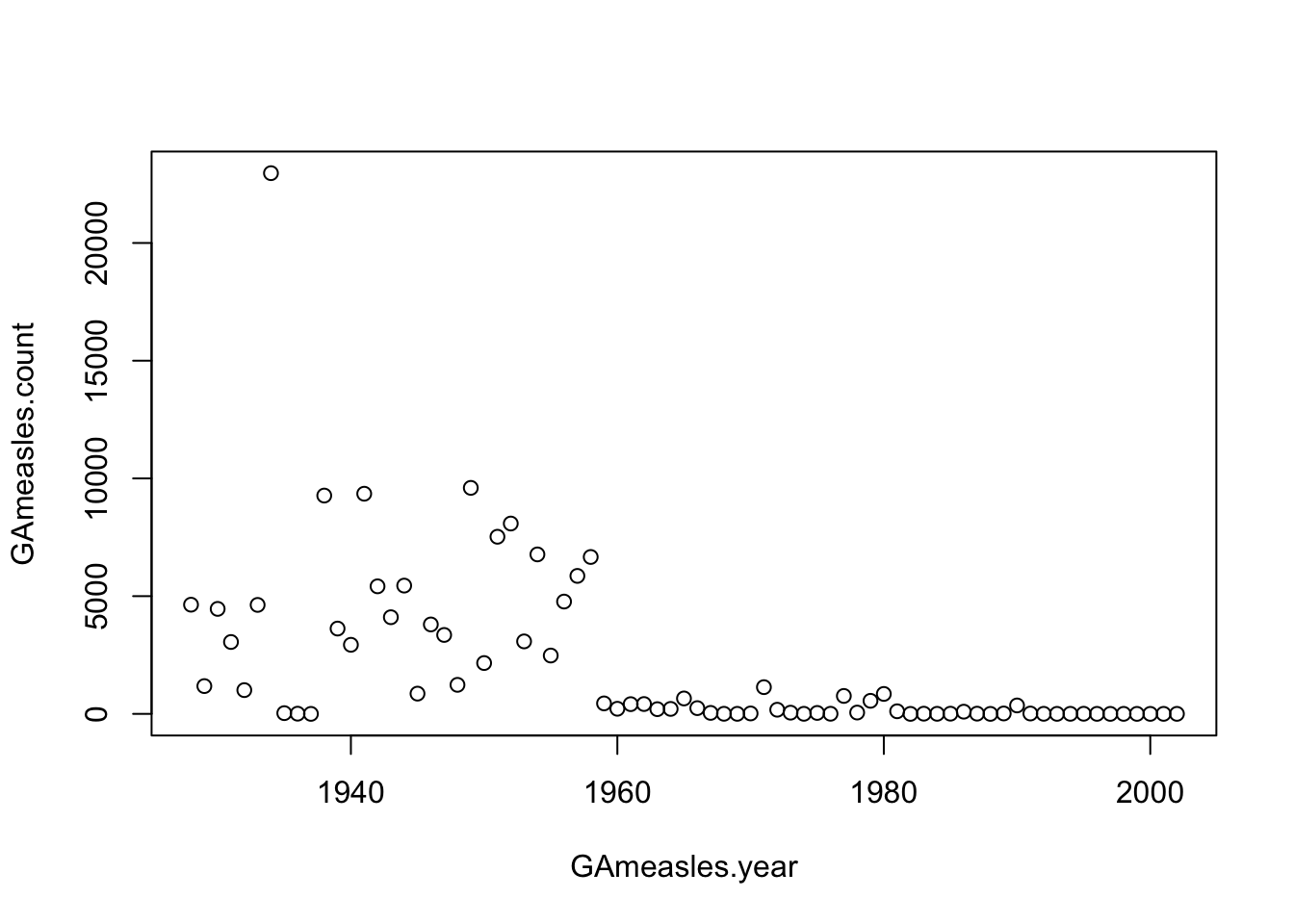
GAmeasles <- subset(us_contagious_diseases,state == "Georgia" & disease == "Measles")
#I wanted to only look at Georgia & Measles data, so I used the filter function and named it GAmeasles.
GAmeasles2 <- data.frame(GAmeasles$year, GAmeasles$count)
#I then created a dataset of year and count for mumps. 
summary(GAmeasles2)

 GAmeasles.year GAmeasles.count  
 Min.   :1928   Min.   :    0.0  
 1st Qu.:1946   1st Qu.:    6.5  
 Median :1965   Median :  244.0  
 Mean   :1965   Mean   : 2073.1  
 3rd Qu.:1984   3rd Qu.: 3215.0  
 Max.   :2002   Max.   :22965.0  

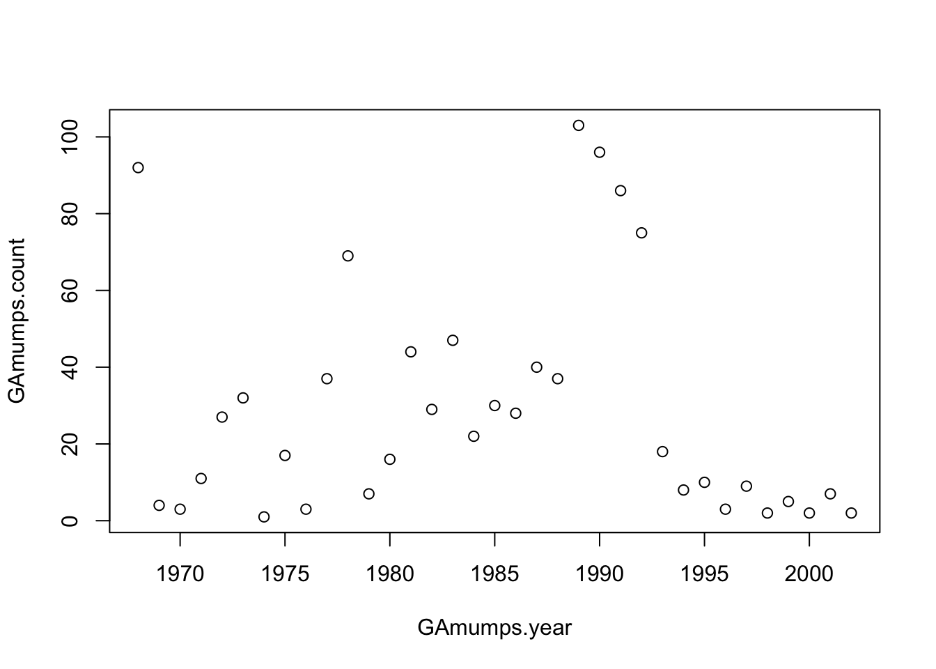
plot(GAmumps2)

#This plot shows an increase from 1970-1989, a spike in 1990, then a decrease. 
plot(GAmeasles2)

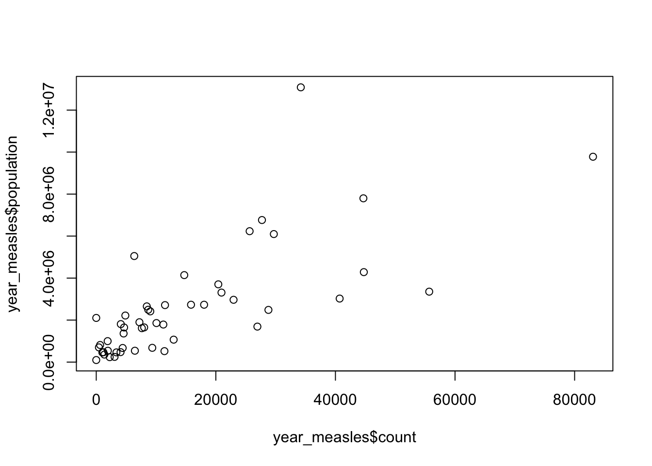
#this plot shows a significant decrease in cases after 1960. 
year_measles <- subset(us_contagious_diseases, (year=="1934" & disease=="Measles"))
#I now used the subset function to only look at measles cases from 2000
plot(year_measles$count, year_measles$population)

#I plotted count of measles cases on the x axis and population of each state on the y axis. 
fit1 <- lm(year_measles$population ~ year_measles$count)
summary(fit1)

Call:
lm(formula = year_measles$population ~ year_measles$count)

Residuals:
     Min       1Q   Median       3Q      Max 
-3852283  -829103  -189625   484704  8305549 

Coefficients:
                    Estimate Std. Error t value Pr(>|t|)    
(Intercept)        909749.73  346349.07   2.627   0.0116 *  
year_measles$count    113.08      15.57   7.264 3.25e-09 ***
---
Signif. codes:  0 '***' 0.001 '**' 0.01 '*' 0.05 '.' 0.1 ' ' 1

Residual standard error: 1806000 on 47 degrees of freedom
  (2 observations deleted due to missingness)
Multiple R-squared:  0.5289,    Adjusted R-squared:  0.5189 
F-statistic: 52.77 on 1 and 47 DF,  p-value: 3.254e-09

#There is a significant positive correlation between population and measles count in 1934.